Introduction
The aim of this study is to predict the birth rate from the data sets of United States Department of Agriculture (Economic Research Service) and the United States’ Census Bureau using different analysis methods. The methods used in the regression problem are linear regression (LM), artificial neural network (ANN), radial, and linear support vector machines (SVMs).
SVMs are dealt with in the supervised learning class of artificial intelligence (AI) and machine learning (ML). In this analysis, ANN method can be considered as DNN (Deep Neural Network) because it has ANN architecture with more than one hidden layer. In the other hand, DNN can be evaluated in the supervised learning class of AI, and in in the field of deep learning (DL).
The results indicate that when Mean Square Error (MSE) and Mean Absolute Error (MAE) error types are compared, the SVM method including the radial basis parameter predicts the birth rates better than the other methods.
Sources of data sets utilized in analysis are given below
- https://www.ers.usda.gov/data-products/county-level-data-sets/download-data/
- https://www.census.gov/data/tables/time-series/demo/popest/2010s-state-detail.html
- https://www.census.gov/data/tables/time-series/demo/health-insurance/acs-hi.2017.htmlNA (Not Available) values are removed from data set.
Data set is consisted of 3141 observations of 11 variables. The variables selected in the analysis are listed below.
- Birth_Rate (Target Variable or Dependent Variable)
- Death_Rate
- Net_Migration_Rate
- Unemployment_Rate
- less_high_school
- high_school
- associate
- bachelor_or_higher
- Poverty_Percent
- Marriage_Rate
- Percent_Uninsured
The procedures and methods used in the analysis are explained step by step in the next sections.
Loading libraries
rm(list=ls())

lapply(c("xlsx","dplyr", "tibble", "tidyr", "ggplot2", "GGally","NeuralNetTools" ,"neuralnet", "formattable", "performanceEstimation", "e1071", "DMwR", "caret"), require, character.only = TRUE)
Loading data set
df <- read.xlsx('data_end_2017.xlsx', sheetName='data')
Defining variables in Tibble and data cleaning
df1<-tibble(Birth_Rate=round(df$Birth_Rate,1), Death_Rate=round(df$Death_Rate, 1),Net_Migration_Rate=round(df$Net_Migration_Rate, 1), Unemployment_Rate=df$Unemployment_Rate,less_high_school=df$V5, high_school=df$V6, associate=df$V7, bachelor_or_higher=df$V8, Poverty_Percent=df$Poverty_Percent, Marriage_Rate=round(df$Marriage_Rate, 1), Percent_Uninsured=df$Percent_Uninsured)

formattable(tibble(ID=1:11, Variables=names(df1))) #Names of variables

str(df1)#3142 observations of  11 variables

df1<-df1 %>% drop_na()#Removing NA (Not Available) values from data set

str(df1)##3141 observations of  11 variables

dim(df1)# Dimensions of data sets: 3141   11

summary(df1)

head(df1)
Names of variables

Data types of variables and number of observations after removing NA values
Classes ‘tbl_df’, ‘tbl’ and 'data.frame':	3141 obs. of  11 variables:
 $ Birth_Rate        : num  11.9 10.9 10.7 12 11.5 12.2 11.7 11.4 10.8 8.4 ...
 $ Death_Rate        : num  9.3 10.1 11.7 9.7 12.4 11.3 13.1 12.6 13.6 13.8 ...
 $ Net_Migration_Rate: num  1 22.5 -25 -3.1 6.4 -21 -5.2 -1.8 2.5 6.9 ...
 $ Unemployment_Rate : num  3.9 4.1 5.8 4.4 4 4.9 5.5 5 4.1 4.1 ...
 $ less_high_school  : num  12.3 9.8 26.9 17.9 20.2 28.6 18.9 16.8 19.1 20.5 ...
 $ high_school       : num  33.6 27.8 35.5 43.9 32.3 36.6 40.4 32.2 38.4 38.2 ...
 $ associate         : num  29.1 31.7 25.5 25 34.4 21.4 24.5 33.1 29.1 28.9 ...
 $ bachelor_or_higher: num  25 30.7 12 13.2 13.1 13.4 16.1 17.9 13.3 12.5 ...
 $ Poverty_Percent   : num  13.4 10.1 33.4 20.2 12.8 34.4 21.3 17.7 18.2 17.2 ...
 $ Marriage_Rate     : num  7 7 7 7 7 7 7 7 7 7 ...
 $ Percent_Uninsured : num  16 16 16 16 16 16 16 16 16 16 ...
Descriptive statistics of variables
   Birth_Rate      Death_Rate    Net_Migration_Rate Unemployment_Rate
 Min.   : 0.00   Min.   : 1.20   Min.   :-68.3000   Min.   : 1.500
 1st Qu.: 9.90   1st Qu.: 8.60   1st Qu.: -5.4000   1st Qu.: 3.500
 Median :11.30   Median :10.40   Median :  0.5000   Median : 4.300
 Mean   :11.38   Mean   :10.27   Mean   :  0.9654   Mean   : 4.598
 3rd Qu.:12.60   3rd Qu.:12.10   3rd Qu.:  7.5000   3rd Qu.: 5.300
 Max.   :28.80   Max.   :21.30   Max.   :150.2000   Max.   :19.600
 less_high_school  high_school      associate     bachelor_or_higher
 Min.   : 1.10    Min.   : 7.30   Min.   : 8.80   Min.   : 4.70
 1st Qu.: 9.00    1st Qu.:30.00   1st Qu.:27.00   1st Qu.:14.70
 Median :12.40    Median :34.80   Median :30.60   Median :19.00
 Mean   :13.81    Mean   :34.42   Mean   :30.56   Mean   :21.21
 3rd Qu.:17.70    3rd Qu.:39.40   3rd Qu.:34.00   3rd Qu.:25.30
 Max.   :58.70    Max.   :54.90   Max.   :46.70   Max.   :78.10
 Poverty_Percent Marriage_Rate   Percent_Uninsured
 Min.   : 3.00   Min.   : 5.50   Min.   : 3.00
 1st Qu.:10.90   1st Qu.: 6.00   1st Qu.:11.00
 Median :14.40   Median : 6.80   Median :15.00
 Mean   :15.38   Mean   : 6.86   Mean   :18.66
 3rd Qu.:18.40   3rd Qu.: 7.10   3rd Qu.:23.00
 Max.   :56.70   Max.   :28.60   Max.   :48.00
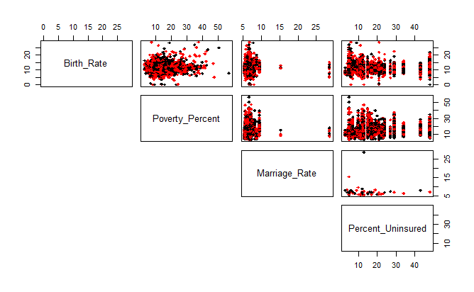
Scatter pair plots of variables: Base mode
pairs(df1[,1:4], pch = 18, cex = 1, col=as.factor(1:3), lower.panel=NULL)

pairs(df1[,c(1,5:8)], pch = 18, cex = 1, col=as.factor(1:3), lower.panel=NULL)

pairs(df1[,c(1,9:11)], pch = 18, cex = 1, col=as.factor(1:2), lower.panel=NULL)
Plot 1: Scatter pair plots of variables: Base mode
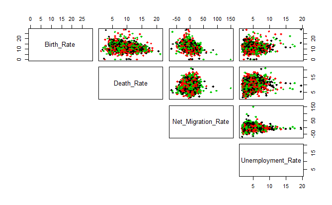
Plot 2: Scatter pair plots of variables: Base mode

Plot 3: Scatter pair plots of variables: Base mode
Scatter pair plots and correlation coefficients: Ggpairs mode
ggpairs(df1[,1:4])
ggpairs(df1[,c(1,5:8)])
ggpairs(df1[,c(1,9:11)])
Plot 1: Scatter pair plots and correlation coefficients: Ggpairs mode

Plot 2: Scatter pair plots and correlation coefficients: Ggpairs mode
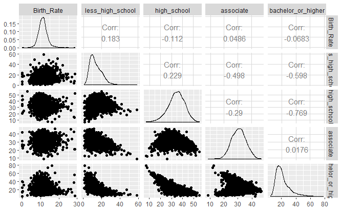
Plot 3: Scatter pair plots and correlation coefficients: Ggpairs mode

Splitting data set into training and test sets
Data set is splitted into training (70%) and test (30%) sets by simple random sampling (SRS) without replacement.
set.seed(1150)
n=NROW(df1)

SRS<-sample(sample(1:n, size = round(0.7*n), replace=FALSE))
training<-df1[SRS,]
test<-df1[-SRS, ]
Building Linear Model (LM) and Predicting
lm.fit <- glm(Birth_Rate~., data=training)
summary(lm.fit)

pr.lm <- predict(lm.fit,test)
Summary of LM
Call:
glm(formula = Birth_Rate ~ ., data = training)

Deviance Residuals:
     Min        1Q    Median        3Q       Max
-12.6431   -1.2701    0.0494    1.2338   17.5226

Coefficients:
                    Estimate Std. Error t value Pr(>|t|)
(Intercept)        -1.210336  86.506626  -0.014    0.989
Death_Rate         -0.196533   0.022653  -8.676  < 2e-16 ***
Net_Migration_Rate -0.040544   0.004030 -10.061  < 2e-16 ***
Unemployment_Rate  -0.069103   0.036281  -1.905    0.057 .
less_high_school    0.238640   0.864714   0.276    0.783
high_school         0.090654   0.865317   0.105    0.917
associate           0.201731   0.865124   0.233    0.816
bachelor_or_higher  0.123188   0.865118   0.142    0.887
Poverty_Percent     0.019001   0.012121   1.568    0.117
Marriage_Rate      -0.012984   0.031243  -0.416    0.678
Percent_Uninsured  -0.022913   0.004762  -4.812  1.6e-06 ***
---
Signif. codes:  0 ‘***’ 0.001 ‘**’ 0.01 ‘*’ 0.05 ‘.’ 0.1 ‘ ’ 1

(Dispersion parameter for gaussian family taken to be 5.620194)

    Null deviance: 14742  on 2198  degrees of freedom
Residual deviance: 12297  on 2188  degrees of freedom
AIC: 10050

Number of Fisher Scoring iterations: 2
Building Artificial Neural Network (ANN) Model
nn<- neuralnet(Birth_Rate ~ Death_Rate + Unemployment_Rate + Net_Migration_Rate+less_high_school+high_school+high_school+associate+bachelor_or_higher+Poverty_Percent+Marriage_Rate+Percent_Uninsured, training, hidden=c(3,2), linear.output=T, threshold=0.01)

summary(nn)

nn$result.matrix#Generating the error of the neural network model

plot(nn)#ANN Architecture

plotnet(nn, cex_val = 1, alpha_val = 1, prune_lty = "dashed")#NN Architecture
Summary of ANN
                    Length Class      Mode
call                    6  -none-     call
response             2199  -none-     numeric
covariate           21990  -none-     numeric
model.list              2  -none-     list
err.fct                 1  -none-     function
act.fct                 1  -none-     function
linear.output           1  -none-     logical
data                   11  data.frame list
exclude                 0  -none-     NULL
net.result              1  -none-     list
weights                 1  -none-     list
generalized.weights     1  -none-     list
startweights            1  -none-     list
result.matrix          47  -none-     numeric
Generating error of ANN model
error                           7.190738e+03
reached.threshold               9.953213e-03
steps                           5.492700e+04
Intercept.to.1layhid1          -1.420848e+00
Death_Rate.to.1layhid1          1.729804e+00
Unemployment_Rate.to.1layhid1   3.007492e-01
Net_Migration_Rate.to.1layhid1 -4.764154e-01
less_high_school.to.1layhid1    8.628385e-01
high_school.to.1layhid1         1.072833e+00
associate.to.1layhid1           1.401955e+00
bachelor_or_higher.to.1layhid1 -1.783482e-01
Poverty_Percent.to.1layhid1    -9.234006e-01
Marriage_Rate.to.1layhid1      -4.927336e-01
Percent_Uninsured.to.1layhid1   2.478482e+00
Intercept.to.1layhid2           2.723703e-01
Death_Rate.to.1layhid2         -1.700317e+00
Unemployment_Rate.to.1layhid2   5.703225e-01
Net_Migration_Rate.to.1layhid2 -2.078499e+00
less_high_school.to.1layhid2   -1.010006e+00
high_school.to.1layhid2         1.714122e+00
associate.to.1layhid2           4.837800e-01
bachelor_or_higher.to.1layhid2  1.039985e+00
Poverty_Percent.to.1layhid2     9.512370e-01
Marriage_Rate.to.1layhid2      -5.561333e-01
Percent_Uninsured.to.1layhid2  -3.077538e-01
Intercept.to.1layhid3          -1.322371e+00
Death_Rate.to.1layhid3         -7.556517e-01
Unemployment_Rate.to.1layhid3   4.942474e-01
Net_Migration_Rate.to.1layhid3 -3.532218e-01
less_high_school.to.1layhid3    1.597219e-01
high_school.to.1layhid3         5.478689e-01
associate.to.1layhid3           1.378378e+00
bachelor_or_higher.to.1layhid3  1.820102e-01
Poverty_Percent.to.1layhid3     1.701603e+00
Marriage_Rate.to.1layhid3      -5.974305e-02
Percent_Uninsured.to.1layhid3   8.631418e-01
Intercept.to.2layhid1          -5.147527e+00
1layhid1.to.2layhid1           -6.029849e+00
1layhid2.to.2layhid1            1.672761e+02
1layhid3.to.2layhid1           -5.579418e+00
Intercept.to.2layhid2           1.244695e+01
1layhid1.to.2layhid2            1.278534e+01
1layhid2.to.2layhid2            1.912635e+00
1layhid3.to.2layhid2            1.174542e+01
Intercept.to.Birth_Rate         4.943155e+00
2layhid1.to.Birth_Rate          3.305572e+00
2layhid2.to.Birth_Rate          3.178053e+00
ANN architecture with two hidden layers

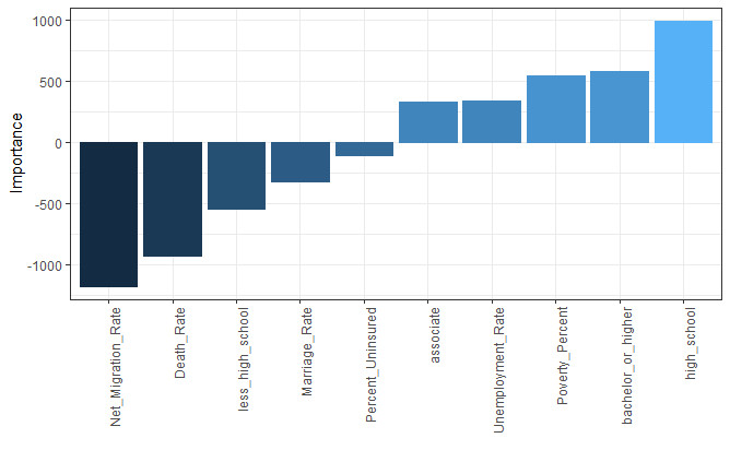
Importance levels of variables in ANN model
In the ANN model, importance levels of variables are calculated using “olden” function because of multiple hidden layers (hidden=c(3,2)), and given below.
olden(nn)+ theme(axis.text.x = element_text(angle = 90, hjust = 1))#Variable importance in ANNs including multiple hidden layers
Importance levels of variables in ANN model
Predicting Birth Rate using ANN
predict_nn <- compute(nn,test[,2:11])
Building SVM (Support Vector Machine) model with Radial Basis parameter, and Prediction
model1 <- svm(Birth_Rate~ ., training, kernel="radial", cost=1, epsilon=0.1, gamma=0.1)

summary(model1)

pred1 <- predict(model1, test)
Summary of SVM with Radial Basis parameter
Call:
svm(formula = Birth_Rate ~ ., data = training, kernel = "radial",
    cost = 1, epsilon = 0.1, gamma = 0.1)


Parameters:
   SVM-Type:  eps-regression
 SVM-Kernel:  radial
       cost:  1
      gamma:  0.1
    epsilon:  0.1


Number of Support Vectors:  1902
Building SVM (Support Vector Machine) model with Linear parameter, and Prediction
model1 <- svm(Birth_Rate~ ., training, kernel="linear")

pred2 <- predict(model1, test)

summary(model1)
Summary of SVM with Linear parameter
Call:
svm(formula = Birth_Rate ~ ., data = training, kernel = "linear")


Parameters:
   SVM-Type:  eps-regression
 SVM-Kernel:  linear
       cost:  1
      gamma:  0.1
    epsilon:  0.1


Number of Support Vectors:  1929
Validation Tests by Methods
1.Cross Validation for LM
r <- performanceEstimation(
PredTask(Birth_Rate ~ .,df1),
workflowVariants(learner = "lm",
learner.pars = list(se = c(0, 0.25, 0.5, 1, 2))),
EstimationTask(metrics = c("mse", "mae"),
method = CV(nReps = 3, nFolds = 10)))
rankWorkflows(r, top = 1)
getWorkflow("lm.v1", r)# AVG MSE: 5.61858 and AVG MAE:1.673429
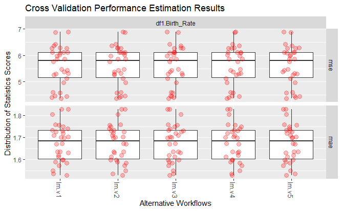
plot(r)
Average MSE, and average MAE for LM model
$df1.Birth_Rate
$df1.Birth_Rate$mse
  Workflow Estimate
1    lm.v1 5.613821

$df1.Birth_Rate$mae
  Workflow Estimate
1    lm.v1 1.674253
Plotting MSE and MAE values for LM model
2. Cross Validation for ANN
#Repeated k-fold Cross Validation
train_control <- trainControl(method="repeatedcv", number=10, repeats=3)

# Train the model
model <- train(Birth_Rate~., data=df1, trControl=train_control, method="nnet")

print(model)
Average MAE for ANN model
It is used Repeated k-fold Cross Validation (NN) as validation test in package “caret” insead of “performanceEstimation” package.
initial  value 403331.122522
final  value 359465.140000
converged
Neural Network

3141 samples
  10 predictor

No pre-processing
Resampling: Cross-Validated (10 fold, repeated 3 times)
Summary of sample sizes: 2827, 2827, 2826, 2827, 2828, 2827, ...
Resampling results across tuning parameters:

  size  decay  RMSE      Rsquared     MAE
  1     0e+00  10.69727          NaN  10.38151
  1     1e-04  10.69727  0.002990157  10.38151
  1     1e-01  10.69729  0.018808431  10.38152
  3     0e+00  10.69727          NaN  10.38151
  3     1e-04  10.69727  0.024056622  10.38151
  3     1e-01  10.69728  0.017597580  10.38152
  5     0e+00  10.69727          NaN  10.38151
  5     1e-04  10.69727  0.011161407  10.38151
  5     1e-01  10.69728  0.022457815  10.38151

RMSE was used to select the optimal model using the smallest value.
The final values used for the model were size = 1 and decay = 0.
3. Cross Validation for SVM (Support Vector Machine) with Radial Basis parameter
pr1 <- performanceEstimation(
PredTask(Birth_Rate ~ .,df1),
workflowVariants(learner="svm",
learner.pars=list(kernel="radial",cost=1, epsilon=0.1, gamma=0.1)),
EstimationTask(metrics = c("mse", "mae"),
method = CV(nReps = 3, nFolds = 10)))
summary(pr1)# AVG MSE:5.0181919 and AVG MAE:1.52361665
rankWorkflows(pr1, top = 1)
getWorkflow("svm", pr1)
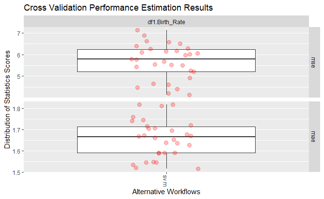
plot(pr1)
Average MSE, and average MAE for SVM (Support Vector Machine) with Radial Basis parameter
-> Task:  df1.Birth_Rate
  *Workflow: svm
              mse        mae
avg     5.0237890 1.52349784
std     0.7941622 0.08445783
med     4.8739686 1.51075518
iqr     0.9747409 0.10690584
min     3.5181964 1.37328251
max     6.4726952 1.71792661
invalid 0.0000000 0.00000000
$df1.Birth_Rate
$df1.Birth_Rate$mse
  Workflow Estimate
1      svm 5.023789

$df1.Birth_Rate$mae
  Workflow Estimate
1      svm 1.523498


Workflow Object:
	Workflow ID       ::  svm
	Workflow Function ::  standardWF
	     Parameter values:
		 learner.pars  -> kernel=radial cost=1 epsilon=0.1 gamma=0.1
		 learner  -> svm
Plotting MSE and MAE values for SVM (Support Vector Machine) with Radial Basis parameter

4. Cross Validation for SVM (Support Vector Machine) with Linear parameter
pr1 <- performanceEstimation(
 PredTask(Birth_Rate ~ .,df1),
 workflowVariants(learner="svm",
                  learner.pars=list(kernel="linear")),
 EstimationTask(metrics = c("mse", "mae"),
                 method = CV(nReps = 3, nFolds = 10)))
summary(pr1)# AVG MSE:5.671183 and AVE MAE:1.6563516

rankWorkflows(pr1, top = 1)

getWorkflow("svm", pr1)

plot(pr1)
Average MSE, and average MAE for SVM (Support Vector Machine) with Linear parameter
##### PERFORMANCE ESTIMATION USING  CROSS VALIDATION  #####

** PREDICTIVE TASK :: df1.Birth_Rate

++ MODEL/WORKFLOW :: svm
Task for estimating  mse,mae  using
 3 x 10 - Fold Cross Validation
	 Run with seed =  1234
Iteration :******************************

== Summary of a  Cross Validation Performance Estimation Experiment ==

Task for estimating  mse,mae  using
 3 x 10 - Fold Cross Validation
	 Run with seed =  1234

* Predictive Tasks ::  df1.Birth_Rate
* Workflows  ::  svm

-> Task:  df1.Birth_Rate
  *Workflow: svm
              mse        mae
avg     5.6742841 1.65745175
std     0.8087646 0.08828428
med     5.7814504 1.66599466
iqr     1.0277489 0.12239844
min     4.1506266 1.51514278
max     7.1174248 1.81856657
invalid 0.0000000 0.00000000
$df1.Birth_Rate
$df1.Birth_Rate$mse
  Workflow Estimate
1      svm 5.674284

$df1.Birth_Rate$mae
  Workflow Estimate
1      svm 1.657452


Workflow Object:
	Workflow ID       ::  svm
	Workflow Function ::  standardWF
	     Parameter values:
		 learner.pars  -> kernel=linear
		 learner  -> svm
Plotting MSE and MAE values for SVM (Support Vector Machine) with Linear parameter
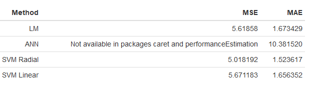
The models built were validated using “performanceEstimation” and “caret” packages. As validation test, Repetitive k-Fold cross validation test (nReps = 3) was used. The MAE and MSE results of the methods used are given in the table 1 below after being presented code block.
Method<-c("LM", "ANN", "SVM Radial", "SVM Linear")
MSE<-list(5.61858, "Not available in packages caret and performanceEstimation",5.0181919,5.671183)
MAE<-c(1.673429, 10.38152,1.52361665,1.6563516)
formattable(tibble(Method=Method, MSE=MSE, MAE=MAE))
Table 1: The MAE and MSE Results of the Methods by Validation Tests
Plotting the results of actual and predicted birth rates by methods
Visual comparison of performance of methods is conducted in terms of actual test values and predicted ones, and were shown below.
#ANN: Comparison of actual and predictive birth rates
results <- data.frame(actual = test$Birth_Rate, predictionNN = round(predict_nn$net.result,1))

#LM: Comparison of actual and predictive birth rates
results1 <- data.frame(actual = test$Birth_Rate, predictionLM = round(pr.lm,1))

#SVM with Radial Basis Parameter: Comparison of actual and predictive birth rates
results3 <- data.frame(actual = round(test$Birth_Rate,1), predictionSVMKernel = round(pred1,1))

#SVM with Linear Parameter: Comparison of actual and predictive birth rates
results4 <- data.frame(actual = round(test$Birth_Rate,1), predictionSVMLinear = round(pred2,1))

comp<-cbind(Birth_Rate=results[,1],NN=results[,2], LM=results1[, 2], SVMRadial=results3[, 2], SVMLinear=results4[, 2])

comparison<-formattable(as_tibble(comp))

plot(test$Birth_Rate,predict_nn$net.result,col='red',main='Real vs predicted NN',pch=18,cex=0.7, xlab="Birth Rate", ylab = "Prediction" )
points(test$Birth_Rate, pr.lm,col='blue',pch=18,cex=0.7)
points(test$Birth_Rate, comparison$SVMRadial,col='brown',pch=18,cex=0.7)
points(test$Birth_Rate, comparison$SVMLinear,col='green',pch=18,cex=0.7)
abline(0,1,lwd=2)
legend("topright",legend=c('NN','LM', 'SVMRadial','SVMLinear'),pch=18,col=c('red','blue', 'brown', 'green'))

Writing results containing actual and predicted birth rates by method into the file with “xlsx” extension
write.xlsx(comparison, file = "comparison_results.xlsx",
           sheetName="results", append=TRUE)
The file called “comparison_results” actual and predicted birth rates by method can be downloaded from the link below.
Showing first ten findings containing actual and predicted values by method
After being presented code block, the first ten rows of actual and predicted birth rates by method used are given in Table 2.
formattable(head(comparison,10))
Table 2: The First Ten Findings Containing Actual and Predicted Birth Rates by Method

Conclusion
As can be seen from the validation test results in the Table 1 above, SVM including Radial Basis Parameter is the best method in terms of MAE and MSE values obtained. Therefore, it is recommended that SVM with Radial Basis Parameter can be used in prediction of birth rates.
Hope to be useful and raise awareness.
Note: It can not be cited or copied without referencing.
Not: Kaynak gösterilmeden alıntı yapılamaz veya kopyalanamaz.
References
- https://www.ers.usda.gov/data-products/county-level-data-sets/download-data/
- https://www.census.gov/data/tables/time-series/demo/popest/2010s-state-detail.html
- https://www.census.gov/data/tables/time-series/demo/health-insurance/acs-hi.2017.html
- https://www.r-project.org/
- https://datascienceplus.com/neuralnet-train-and-test-neural-networks-using-r/
- http://cs229.stanford.edu/notes/cs229-notes3.pdf
- http://www.cs.columbia.edu/~kathy/cs4701/documents/jason_svm_tutorial.pdf
- http://svms.org/tutorials/BurbidgeBuxton2001.pdf
- https://course.ccs.neu.edu/cs5100f11/resources/jakkula.pdf
- https://med.nyu.edu/chibi/sites/default/files/chibi/Final.pdf
- http://ijarcet.org/wp-content/uploads/IJARCET-VOL-1-ISSUE-10-185-189.pdf
- http://www.ijastnet.com/journals/Vol_7_No_2_June_2017/2.pdf
- https://www.demographic-research.org/volumes/vol20/25/20-25.pdf
- https://www.hindawi.com/journals/cmmm/2013/487179/
- http://www.cinc.org/Proceedings/2005/pdf/0247.pdf
- https://scialert.net/fulltext/?doi=jai.2016.33.38
- https://papers.ssrn.com/sol3/papers.cfm?abstract_id=2894370
- https://www.ijeat.org/wp-content/uploads/papers/v9i1/A9386109119.pdf
- https://www.ijitee.org/wp-content/uploads/papers/v8i9S/I11460789S19.pdf
- https://biomedpharmajournal.org/vol11no3/emg-signal-analysis-for-diagnosis-of-muscular-dystrophy-using-wavelet-transform-svm-and-ann/
- https://canvas.harvard.edu/courses/12656/files/3151019/download?verifier=62k2w6mW3Glg0caFIRHfXACHlC0iS5JzwJTfTZZr&wrap=1
- https://scholar.harvard.edu/files/javierzazo/files/svms.pdf